1. Task - Exterior wall with connecting interior wall
This tutorial shows how 2D details of constructions can be simulated with DELPHIN. For this purpose, a simple thermal bridge is modelled and calculated. This tutorial refers to DELPHIN versions from 6.1.5.
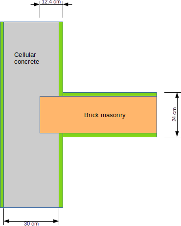
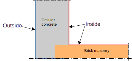
The constructional detail shown below represents an interior wall that ties into an exterior wall and is to be calculated in DELPHIN. The exterior wall is made of aerated concrete, the interior wall is a brick masonry.
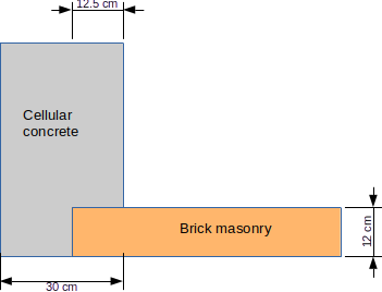
1.1. Simplification of the construction details
Before a construction is entered into DELPHIN, it should be examined whether the model can be simplified. In this example, the plaster layers and mortar layers are neglected. Another possibility is to use symmetry axes and choose the model boundary along this axis. This will reduce the number of discretised elements and thus the simulation time.
1.2. Generating the construction grid
In DELPHIN, constructions are developed in a rectangular grid. First, the construction lines are defined, then materials are assigned to the individual fields, or they remain empty, as in the case of a hole, for example. The following grid shows the (simplified) construction:
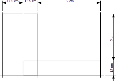
For the length/width marked '? cm', values are still needed. The modelled length of the outer and inner wall must be chosen so large that the influence of the thermal bridge on the temperature field is no longer relevant. According to EN 10211, a length of one metre or three times the thickness of the wall, whichever is greater, should be used here. Here, 60 cm is chosen for the outer wall and 50 cm for the inner wall. If it becomes obvious from the simulation results that the ends of the one-dimensional wall cross-sections are still influenced by the thermal bridge, the detail should be chosen larger.
2. Input in DELPHIN
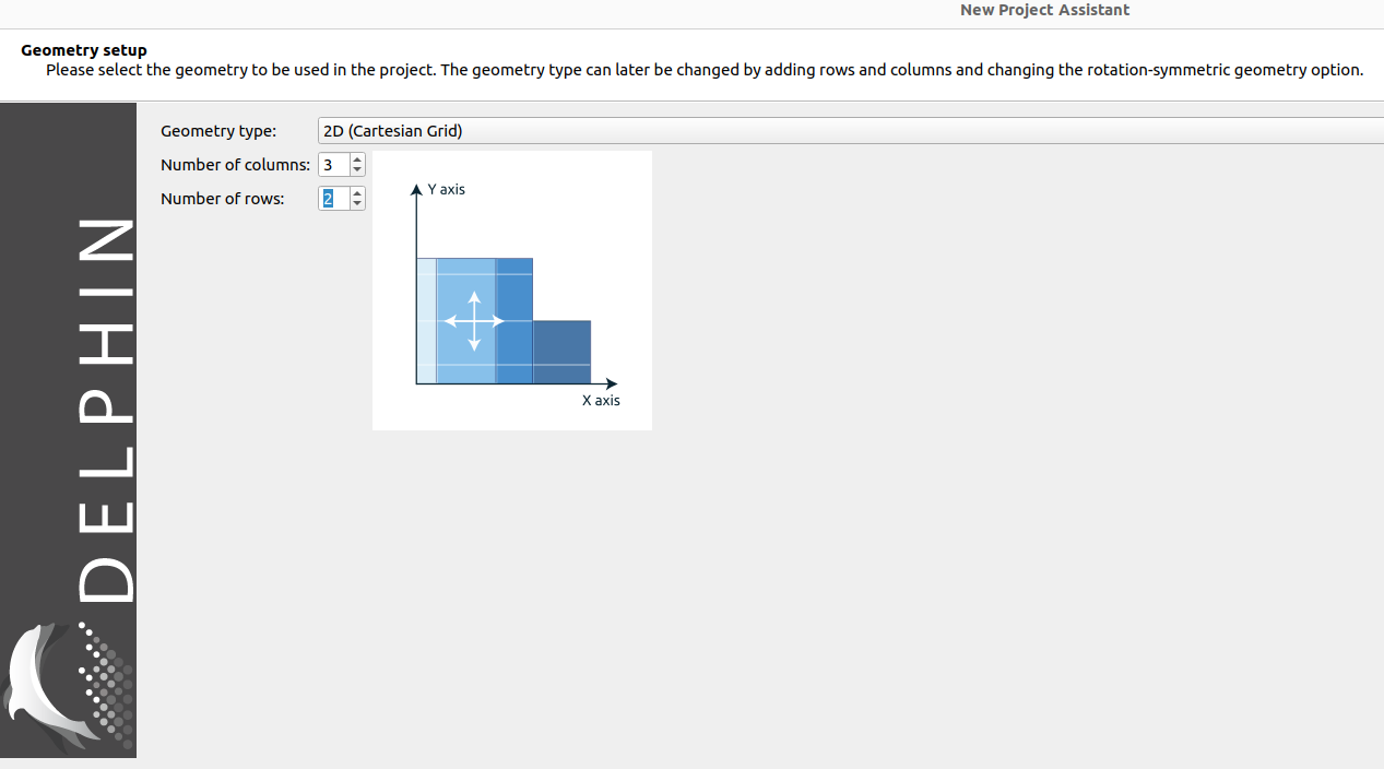
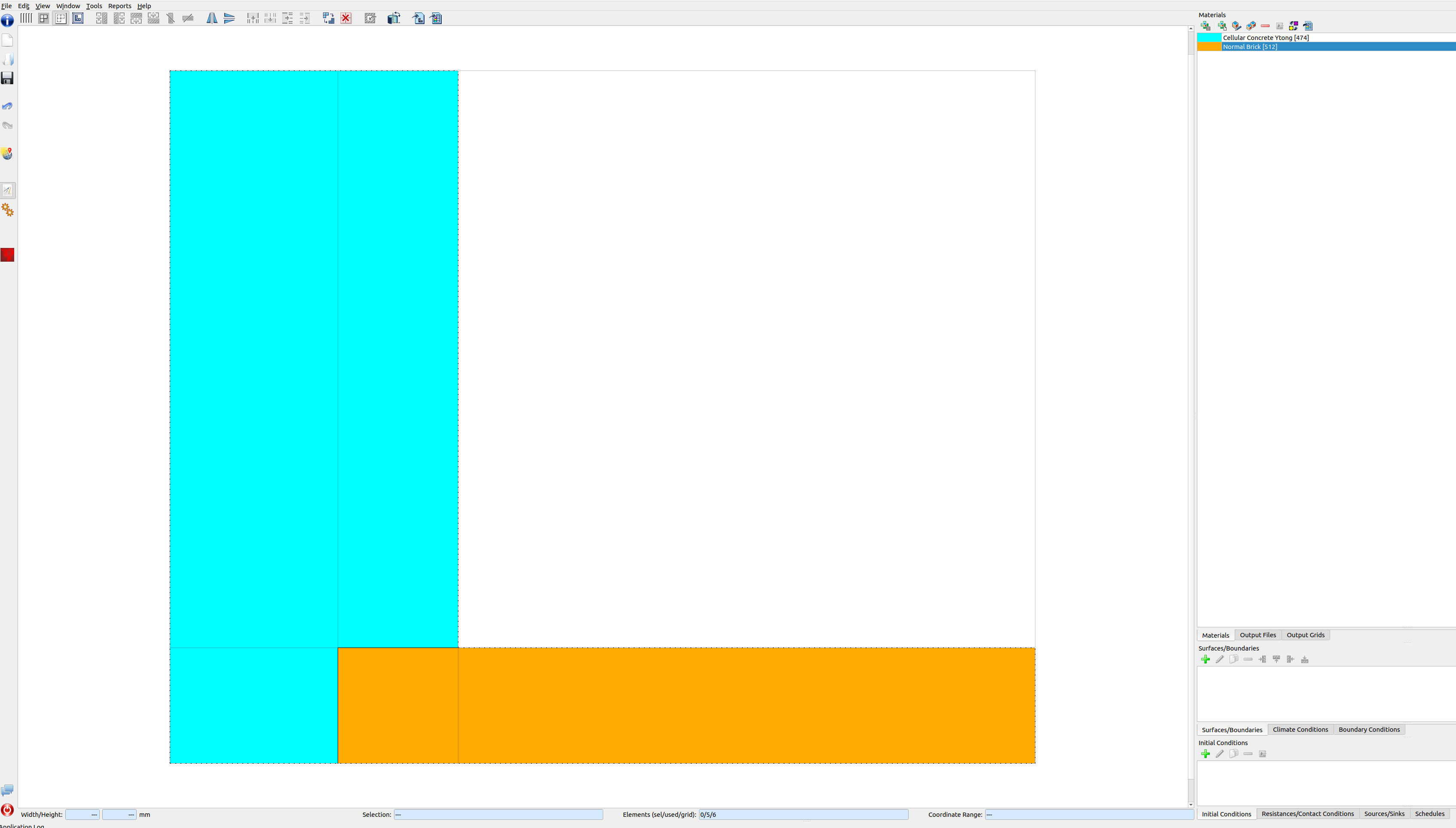
The modelling procedure is analogous to tutorial 1. When creating the project, the project information should be left blank here. A hygrothermal simulation (standard) is selected and the calculation period is set to 2 years. Potsdam is to be selected as the climate location. For the materials, any aerated concrete (e.g. 474) and a standard brick (e.g. 512) can be selected. Afterwards, '2D (Cartesian coordinate system)' should be selected in the geometry default window. Here you already enter the column and row numbers from the construction grid. Layer thicknesses or heights can be easily changed later, as well as new layers can be added or deleted.
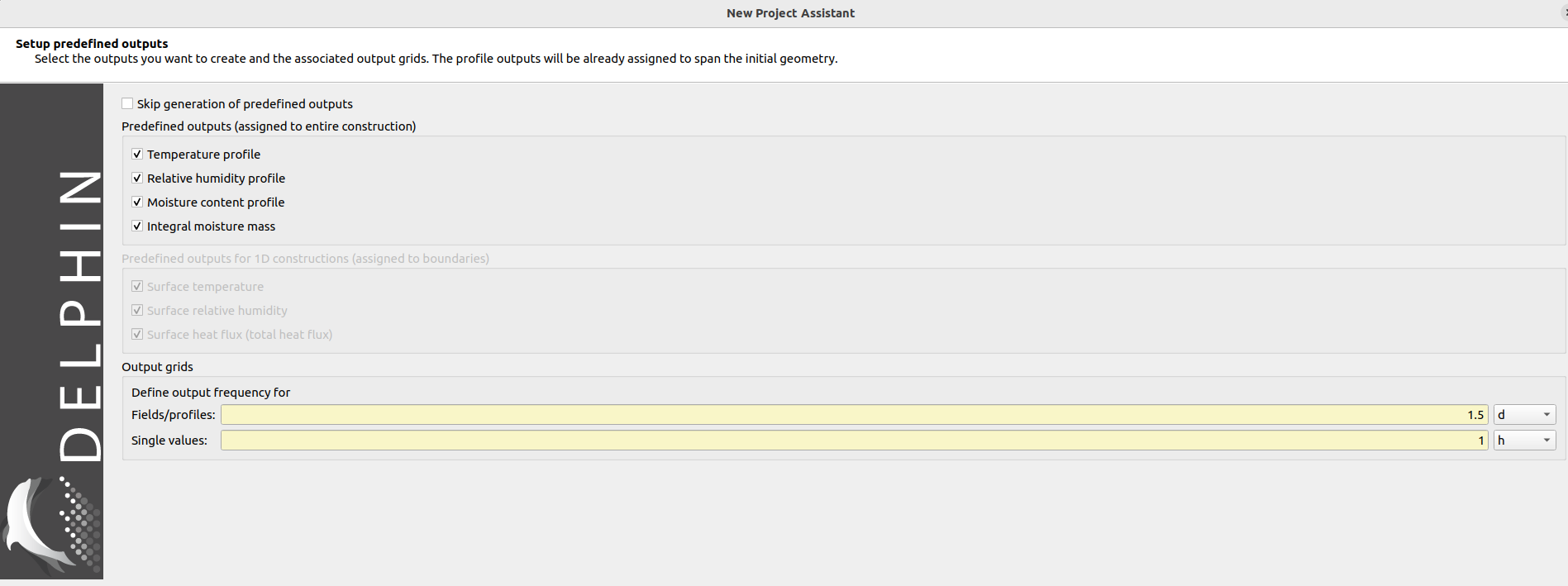
The next dialogue is for creating and assigning surfaces. Since 2D constructions do not always have a clear assignment to inside and outside, this dialogue is displayed but not executed. In the following dialogue, basic outputs are suggested, which are retained. Later, additional outputs can be defined and assigned at any time.
Since no automatic assessment is possible for 2D calculations, the evaluation dialogue is skipped. After finishing the project wizard the grid is displayed in the geometry view.
Now the correct values for the column and row widths are entered, for example, for the bottom left element the width in the edit field is 175 mm. By default all columns and rows are set to 100mm. It works like this:
-
Click on an element of the row or column to be changed.
-
Change width or height in the input fields of the footer at the bottom left.
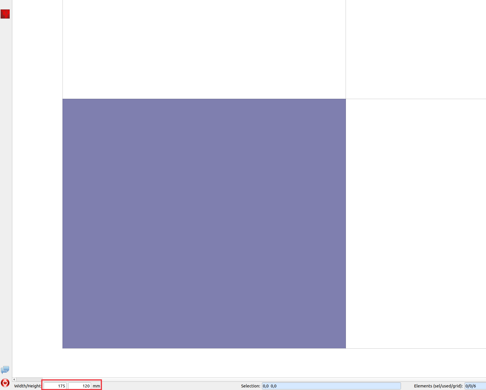
Afterwards, the other dimensions can be adjusted accordingly.
In the following, assignments will be explained in more detail. Assignments can be made for individual elements or entire areas. The elements can be selected with the mouse or keyboard in the construction. In the footer of the construction window the currently selected elements (element numbers) are always displayed, e.g. selection: 0,0….1,1 (DELPHIN always starts with 0).
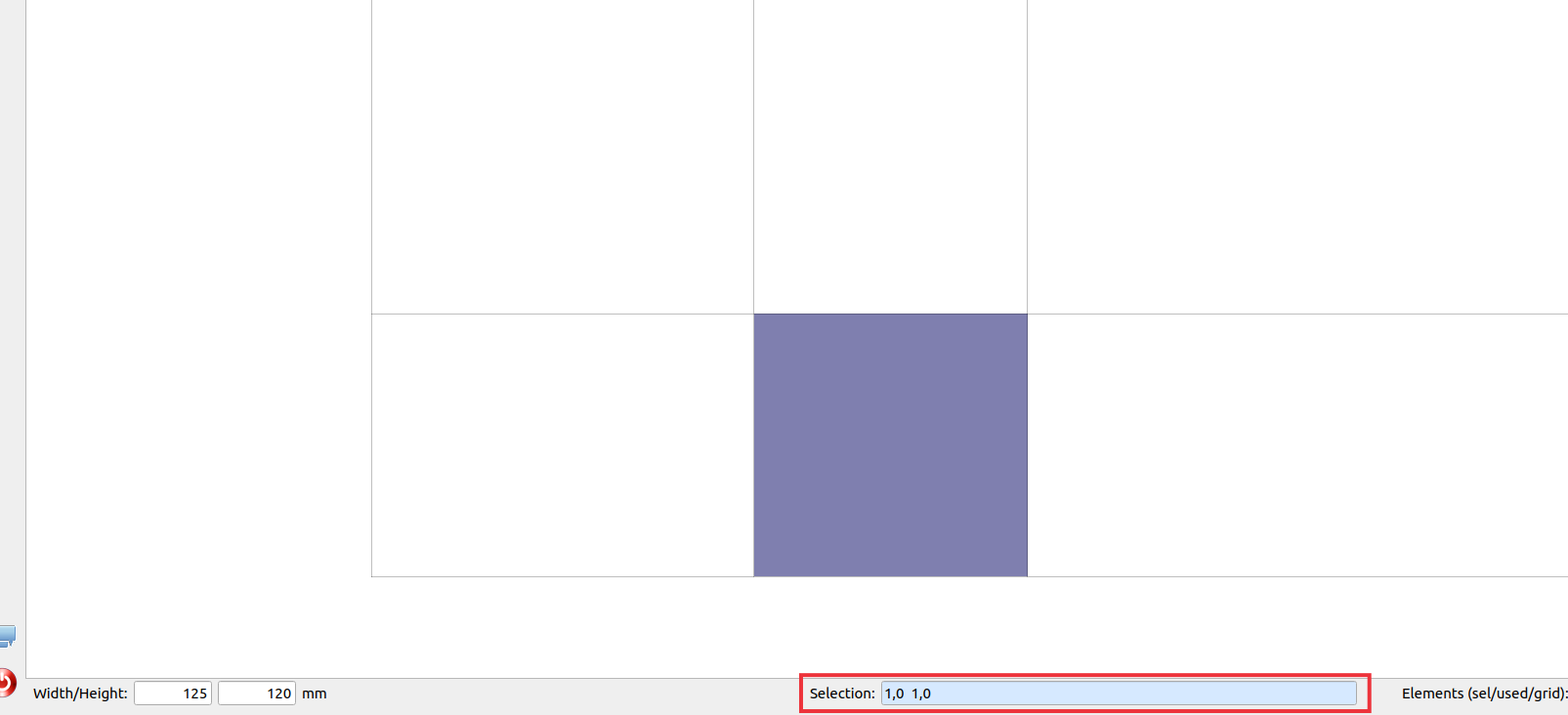
This is equivalent to a range starting from the lower left element with coordinates x=0 and y=0 to the element with coordinates x=1 and y=1, thus covering 4 elements. The numbering of the elements always starts in the lower left corner.
For 2D constructions there are several possibilities to assign materials to areas:
-
Successive selection of elements and assignment of specific materials, which can be very time-consuming for complex 2D details.
-
Selecting larger areas and taking advantage of the fact that previous assignments are automatically overwritten. In this example, cellular concrete is assigned to the area 0.0 … 1.1. Then the brick is assigned to the elements 1.0 … 2.0. In the process, the element 1.0, which was previously assigned aerated concrete, is now assigned the brick.
The second option usually allows a much faster development of the geometric model. In DELPHIN, only the last assigned material is used.
There is also a special type of "material assignment", which is intended for corners or cavities in constructions. In the upper toolbar of the construction window, a button can be used to define elements that have already been assigned a material as an empty area. This overwrites previous assignments. Such an area is actually regarded as empty by DELPHIN, not even as air space. Therefore, climatic boundary conditions can be assigned there at the edges.
An air-filled area can be generated in a construction if elements are assigned the "material" air from the database, analogous to the procedure for assigning materials.
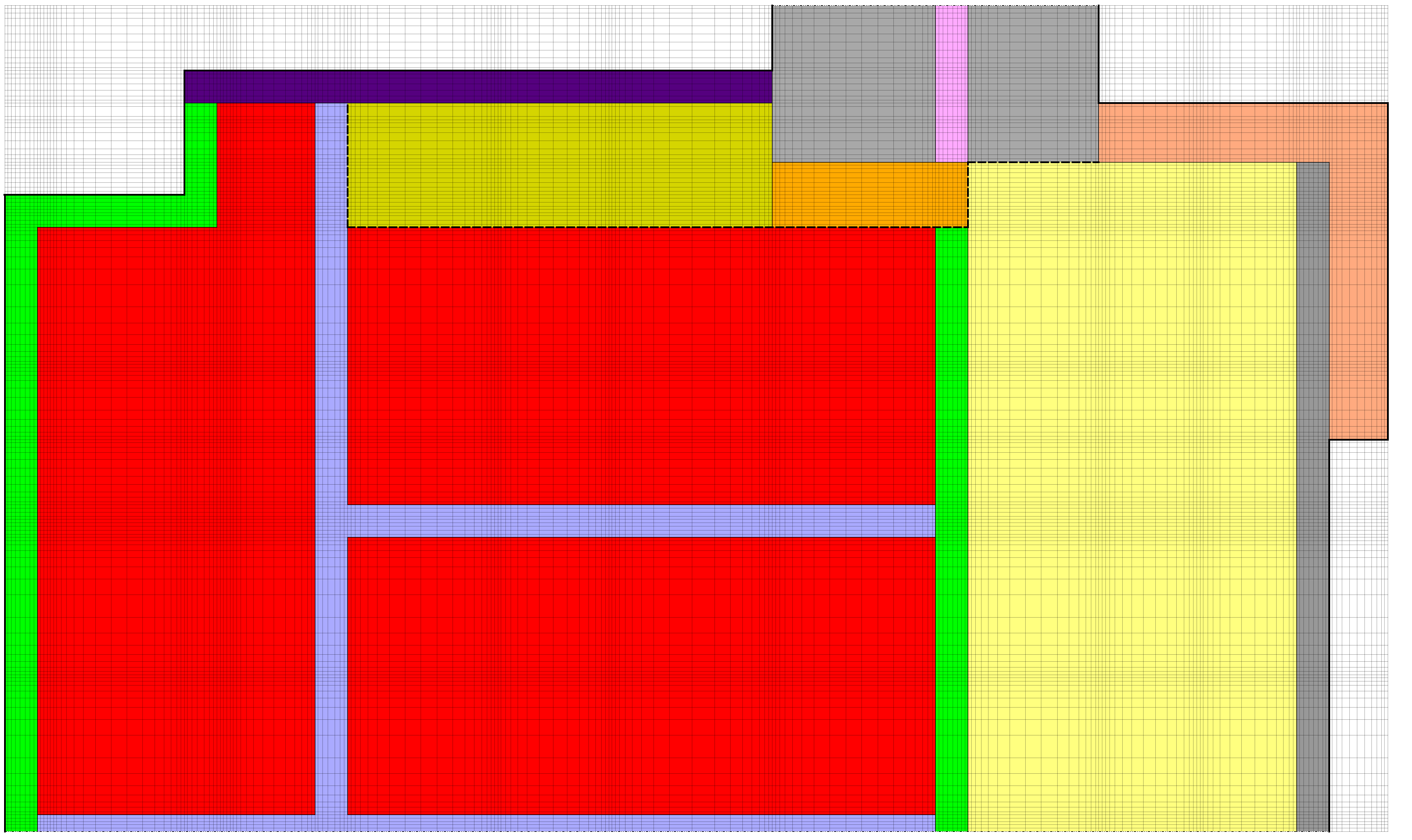
If an assignment is to be deleted or changed, it is better to remove the corresponding assignment in the assignment list (drag the lower edge of the material window upwards). The following picture shows the construction with assigned materials.
3. Assigning surface conditions or climatic boundary conditions
In this chapter surface conditions are assigned to some edges of the modelled construction. The following sketch illustrates the boundary conditions and the associated climatic conditions for temperature and relative humidity at the surfaces.
Boundary conditions are not necessary at symmetry axes and edges of the computational domain where one-dimensional conditions are expected. An edge without climatic boundary condition is treated as absolutely dense and adiabatic. Boundary conditions for heat and steam are to be generated and assigned for the other two boundaries.
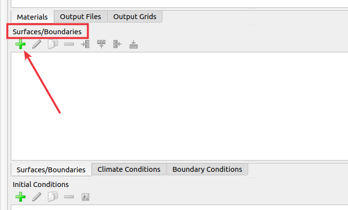
Two surfaces/edges must be defined: one for the indoor climate and one for the outdoor climate. The project wizard enables the local assignment of the outdoor climate. Then create a new surface by clicking on the green plus in the surface list.
The outdoor climate conditions should be selected in the same way as the entries below.
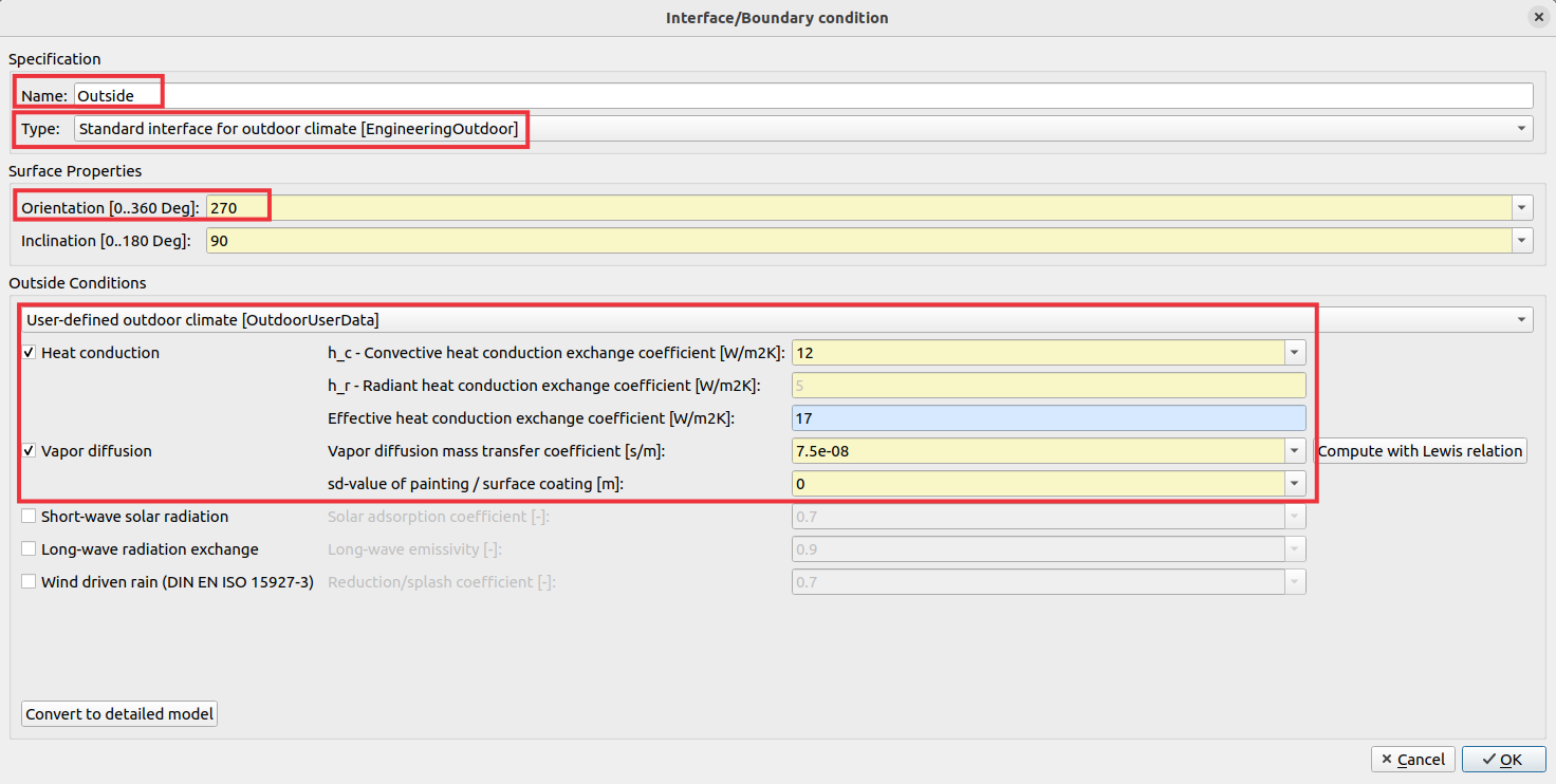
The following settings will be adjusted:
-
Name to 'Exterior'
-
Type - 'Standard Outdoor'.
-
Orientation - 270 (West)
-
Type of outdoor condition - 'User-defined outdoor climate
-
Tick heat conduction and vapour diffusion.
Driving rain and radiation are neglected here.
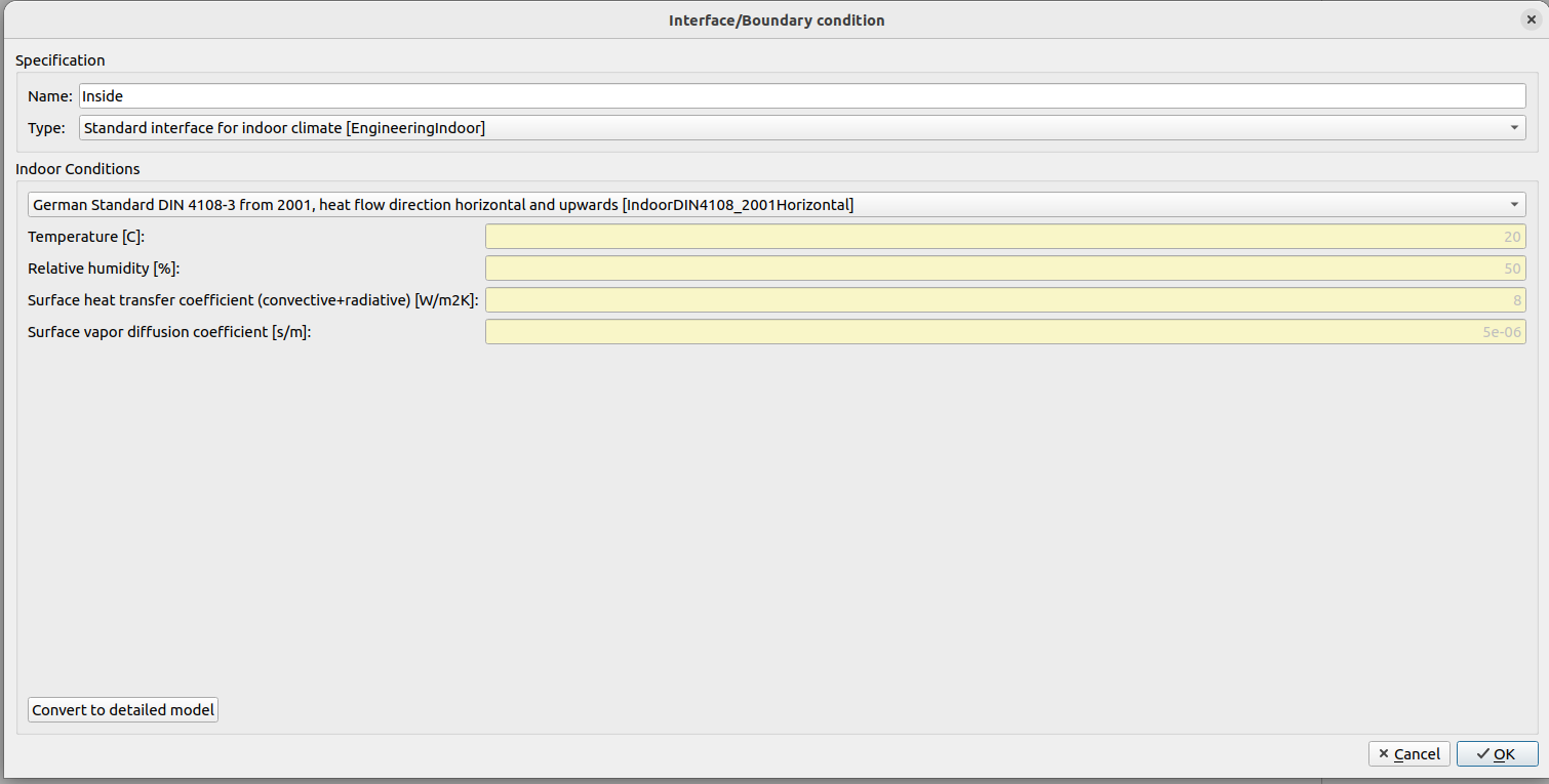
For the indoor climate, constant boundary conditions as in DIN 4108-2 are selected.
The assignment is made as described in Tutorial 1:
-
Select the elements to which the boundary condition is to be assigned.
-
Selecting the condition from the Surface/Margin window.
-
Assigning the surface/margin by selecting the correct assignment button.
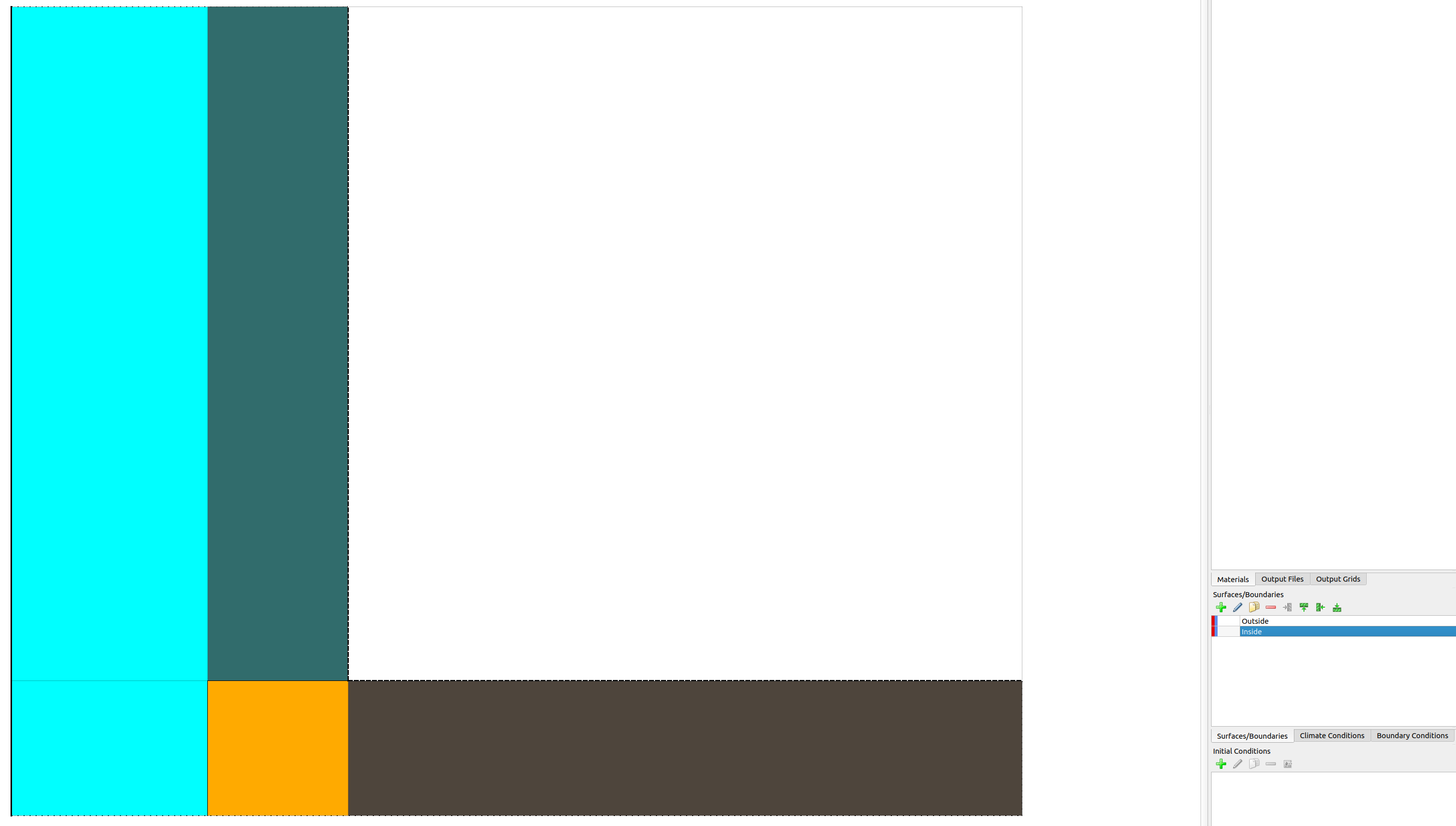
The following screenshot shows how to assign the climatic boundary condition (surface) to the inner surface.
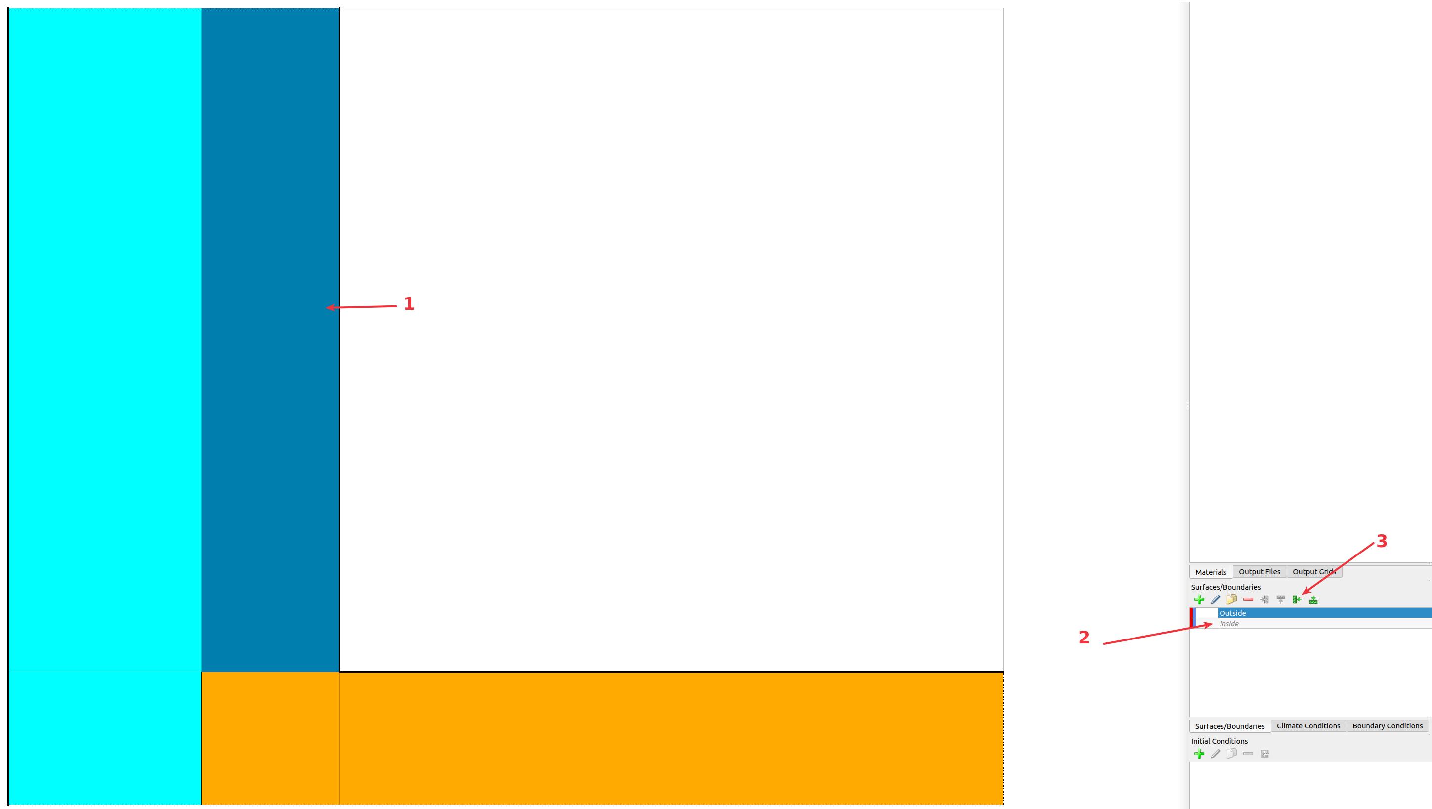
When all boundary conditions or surfaces have been set, the correct assignment can be checked by clicking on a condition in the Surfaces/Borders window. For example, after clicking on 'Indoor climate', all room surfaces are highlighted by a dashed line.
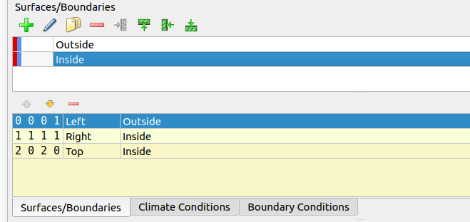
In the assignment list of the window Surfaces/Borders (drag the lower border upwards) each individual assignment can be checked. Three assignments should now be visible here.
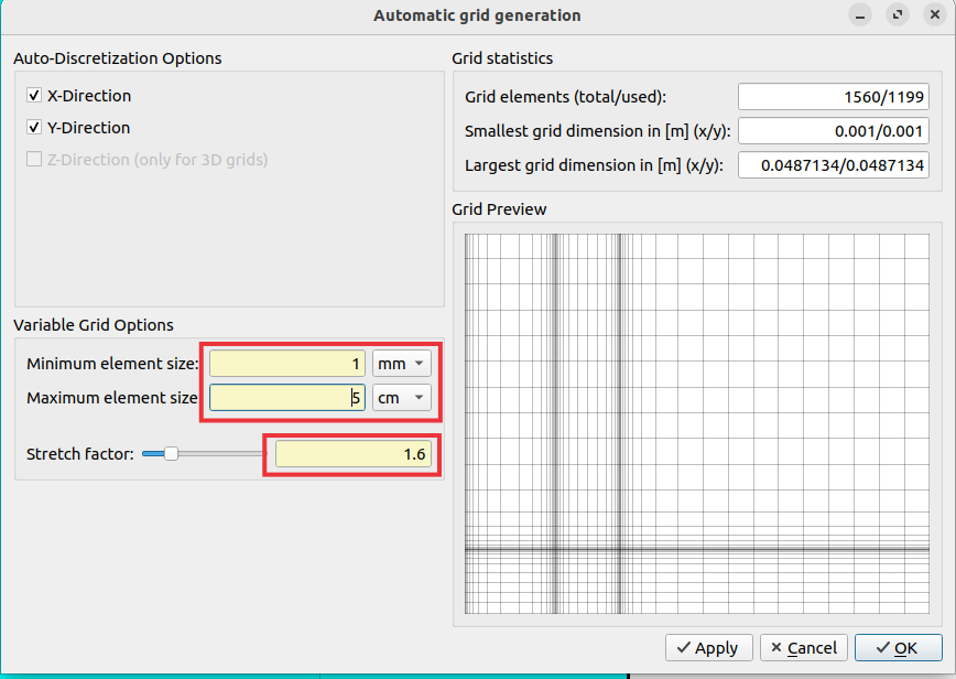
4. Generation of the discretisation grid
After creating the construction and assigning materials and boundary conditions, the grid for the discretisation has to be generated. This is most easily done with the dialogue for automatic discretisation . In this dialogue, both discretisation directions x and y (default for 2D constructions) must be clicked for this thermal bridge. For the minimum element thickness, 1 millimetre is a good value that should only be exceeded slightly. Here, 50 mm is selected for the maximum element thickness with a scaling factor of 1.6.
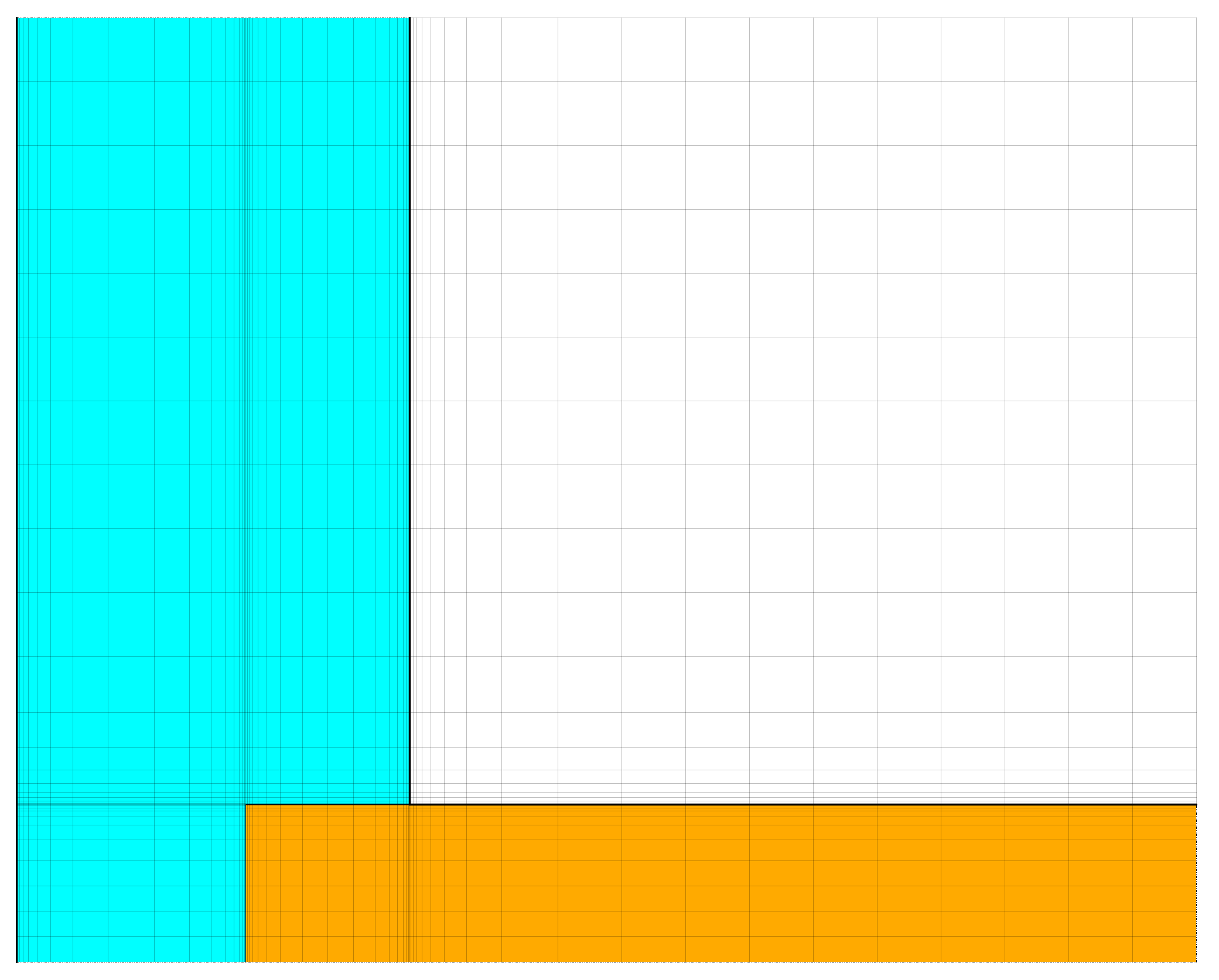
After discretisation the grid looks like this:
Here are some remarks about the different functions of the status bar in the footer of the construction grid.

The status bar contains various information when one or more elements are selected:
-
At 'Width/Height' the total height and width of all selected elements are shown. In this field, the width and height of each individual field can also be changed. However, this function is deactivated if several fields are selected.
-
In 'Selection' there are three numbers: the first indicates the number of elements currently selected, the second indicates the number of cells to which material has been assigned and the third indicates the number of all cells.
-
Selection' and 'Coordinate Range' list the number and coordinates of the currently selected elements, respectively, starting with the first element in horizontal direction, then the first selected element in vertical direction, starting from the bottom left. This is followed by the last element in horizontal direction and finally in vertical direction (DELPHIN starts at '0', not '1').
The automatic discretisation generates a grid that is more finely discretised towards the edges, i.e. towards the construction surfaces (climate) and material boundary layers. Therefore, it is easier to assign surface conditions before discretisation.
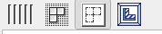
The above buttons, at the top left of the construction window, change the display of the geometric model on the screen. Thus it is possible (from left to right) to switch between proportional and equidistant representation of the elements, to show and hide construction lines, to show and hide the lines of the discretised elements and a button to fit the whole construction optimally into the window.
5. Outputs
For a simple thermal bridge, the temperature field is only used for a rough visual analysis, e.g. to identify the area with the lowest temperatures. On the other hand, temperatures and relative humidities in critical areas, especially the interior wall surfaces, are important for the constructive design of a detail and for the verification in accordance with the guidelines. In addition, heat flows over the interior surface can be interesting for quantifying heat losses in the area of thermal bridges. The postprocessor allows to visualise and evaluate temperatures and other variables at specific points as well as profiles along section lines in a time-resolved manner. In this example, the temperature field is to be generated first. Likewise, given existing data (time series of temperature and relative humidity), the probability of mould formation can be calculated.
The project wizard contains some predefined outputs. In this case these are:
-
Temperature, humidity and water content profiles or fields.
-
Moisture mass integral
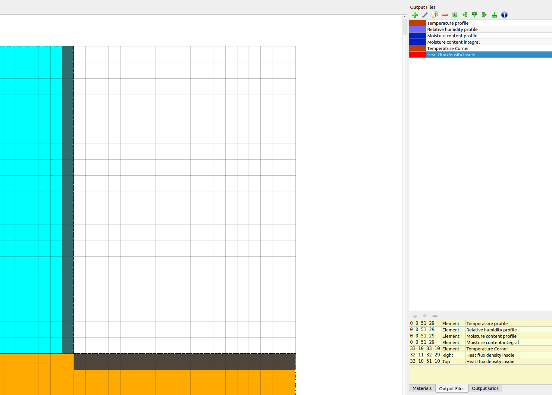
In the field 'Output files' a variety of own outputs can be defined. The following screenshot shows the definition for the averaged temperature output [Mean] in a range or a specific point. It is useful to define the name so that it is clear what exactly is being saved.
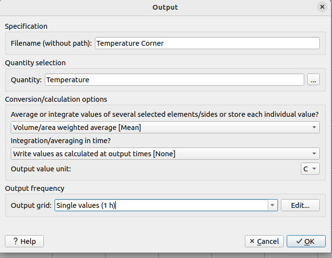
An output for relative humidity can be created in the same way. It is somewhat quicker to simply copy the temperature output that has just been generated. Both outputs should be assigned to the critical point of the construction, the inner corner. Since the discretised elements are quite small, it is usually more convenient to choose the equidistant representation to assign the outputs to individual elements.
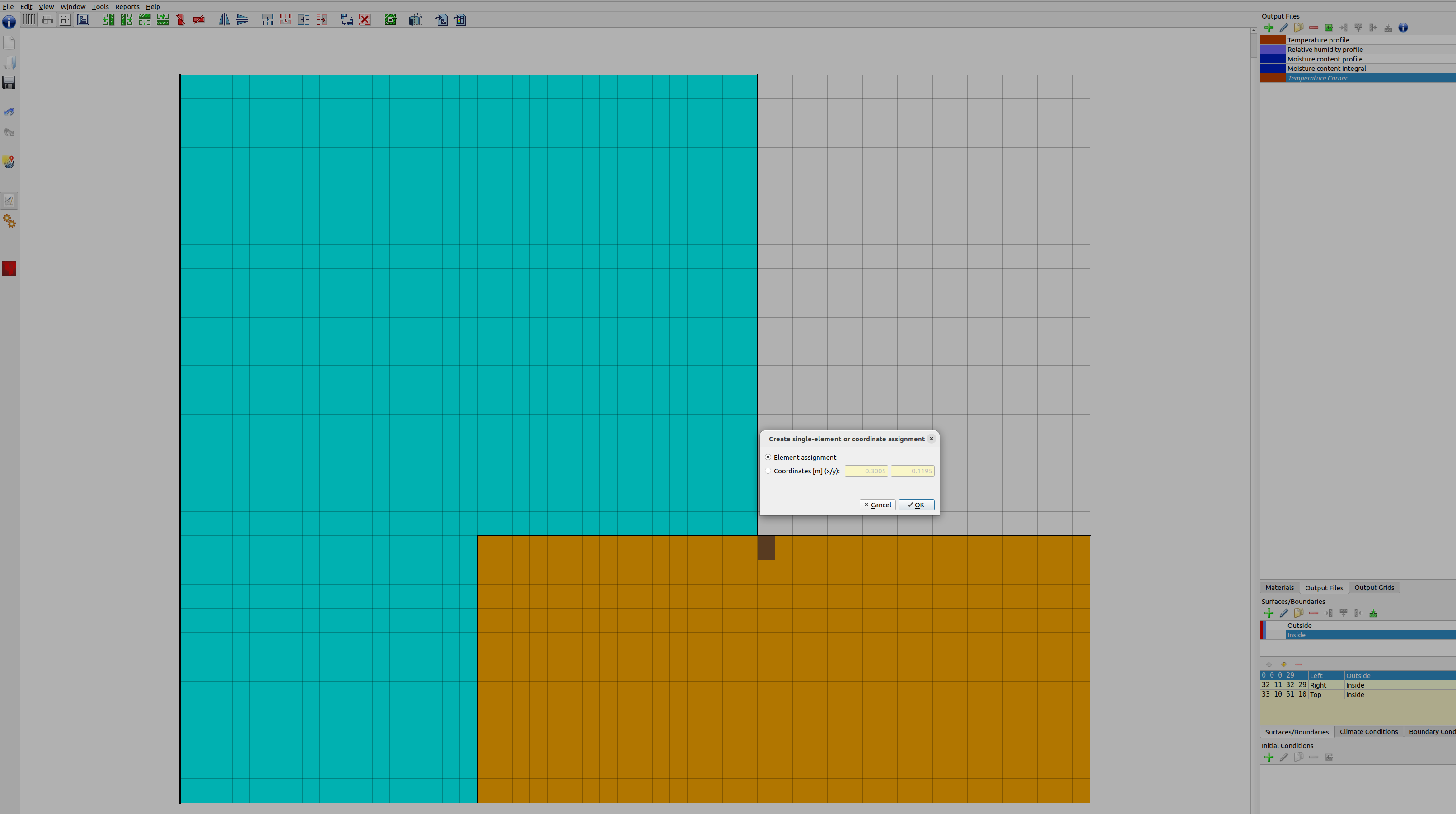
DELPHIN offers the possibility to assign outputs to an element(s) or coordinates. Here the outputs are assigned to a single element. The next output is defined for the heat flow. In this case, two outputs are necessary.
There are two different definitions to consider for flux outputs:
-
Flows at construction edges are positive for inflowing and negative for outflowing.
-
Flows in the field (i.e. inside the construction) are dependent on direction (see below).
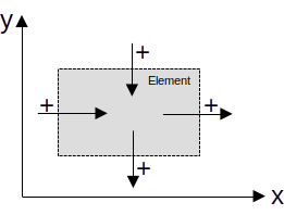
If a selection contains both field elements and elements on edges, the definitions for the field conditions are used. It is also possible to assign a flux output to different element pages. In this case, the assignment is done successively for both sides. In the case of an area/volume-averaged output definition, the area/volume-averaged value is then output for both sides, e.g. at edges. In such a case, you first create the output and then assign it to different margins one after the other.
Here such a boundary condition has been generated for the heat flow over the inner surface:
6. Evaluation - Post-processing
More information about the post-processor can be found in tutorial 3. The following is a short overview of the post-processor PostProc 2 (>> File >> Settings >> External Programs). The next picture shows the temperature field on 15 January in non-interpolated raw data mode (top) and in the interpolated mode (bottom). In the non-interpolated mode the discretised elements stand out clearly.

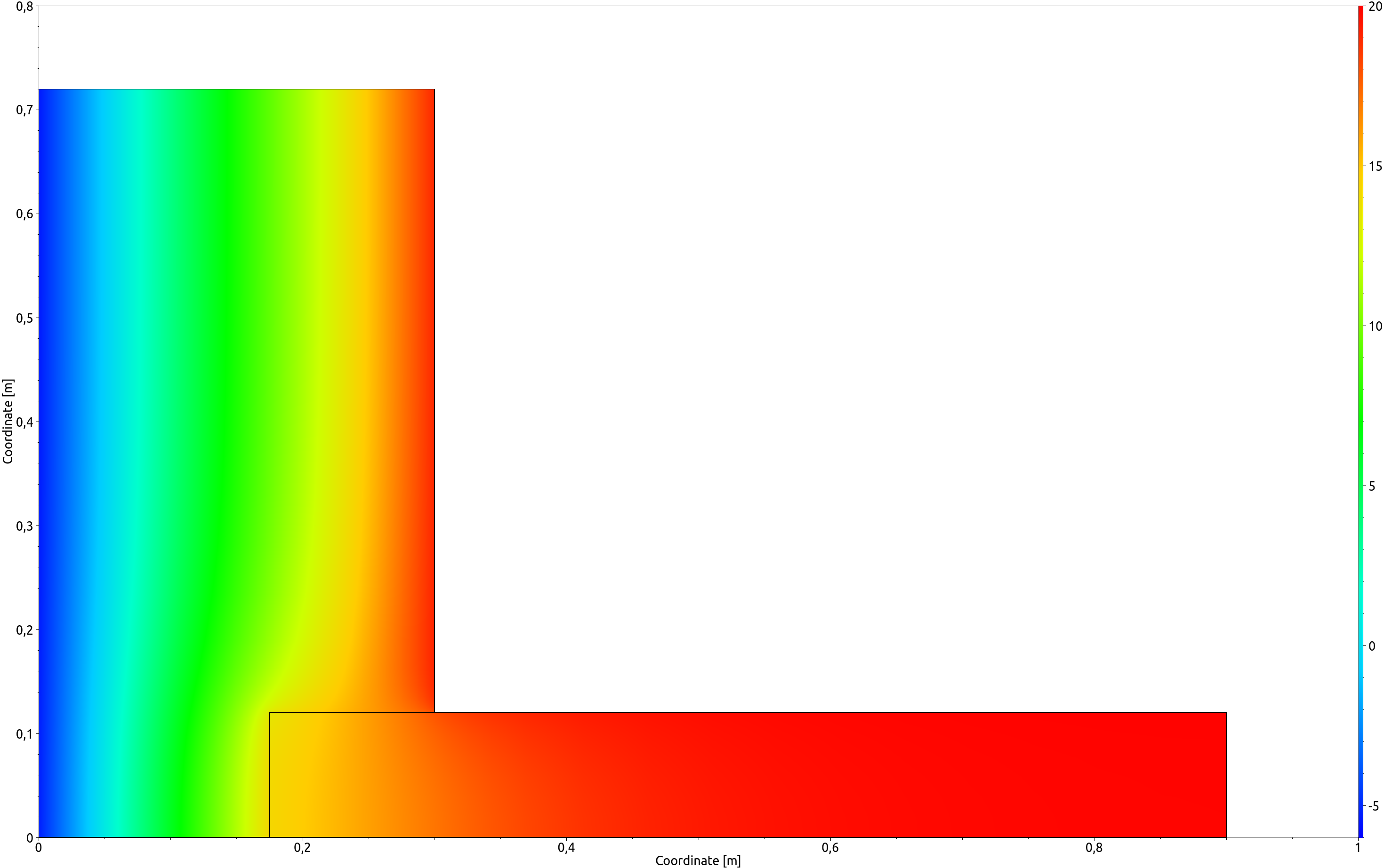
The temperature field with isotherms and color bands for the same time is shown in the next figure.
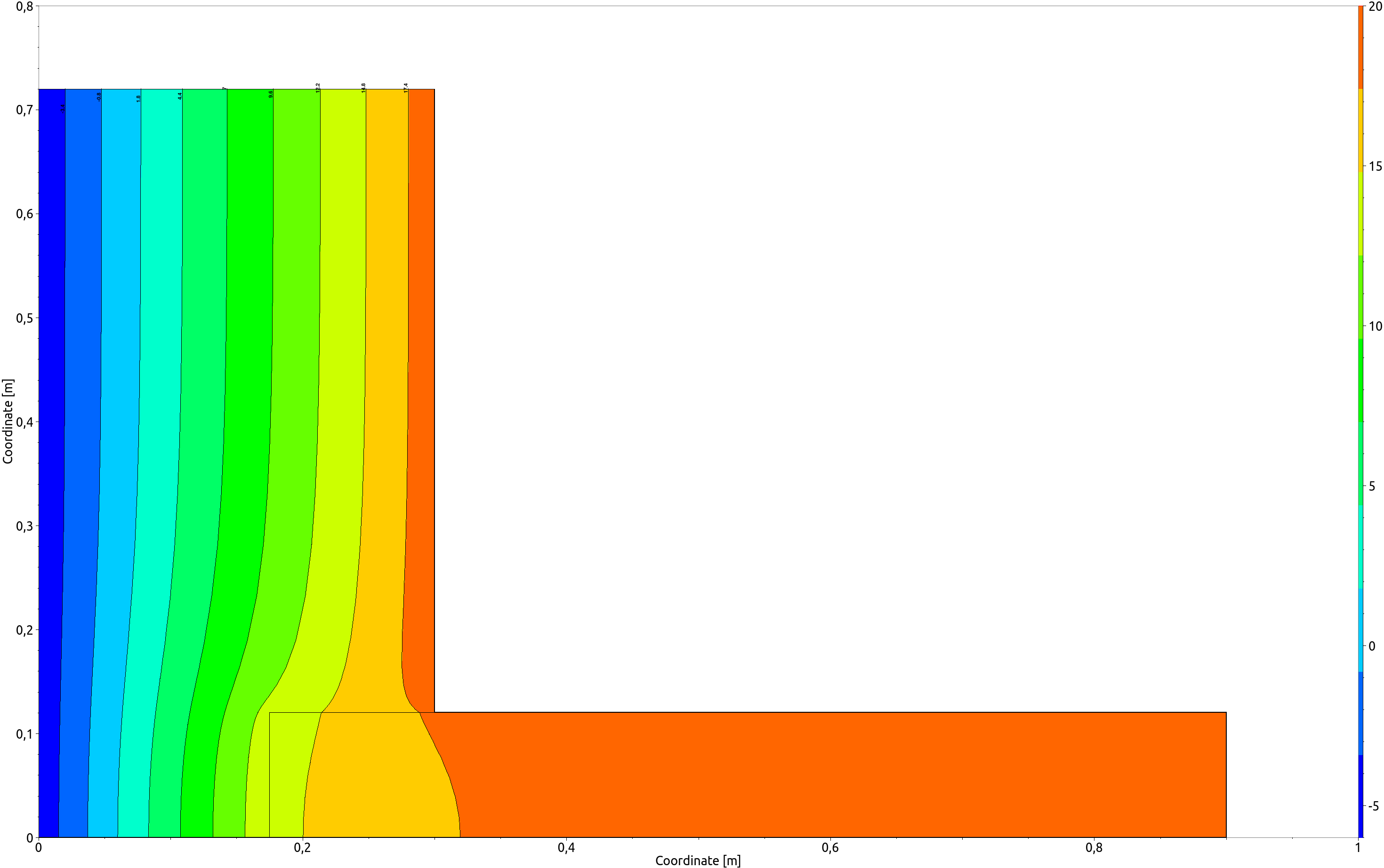
These types of plots allow, for example, to estimate whether the selected wall lengths reach the undisturbed area. For the inner wall this is the case very quickly, whereas for the outer wall it is just sufficient.
The DELPHIN post-processor also allows the use of two y-axes with different units. The next (edited) figure contains the temperature and humidity at the critical point, the inner corner.
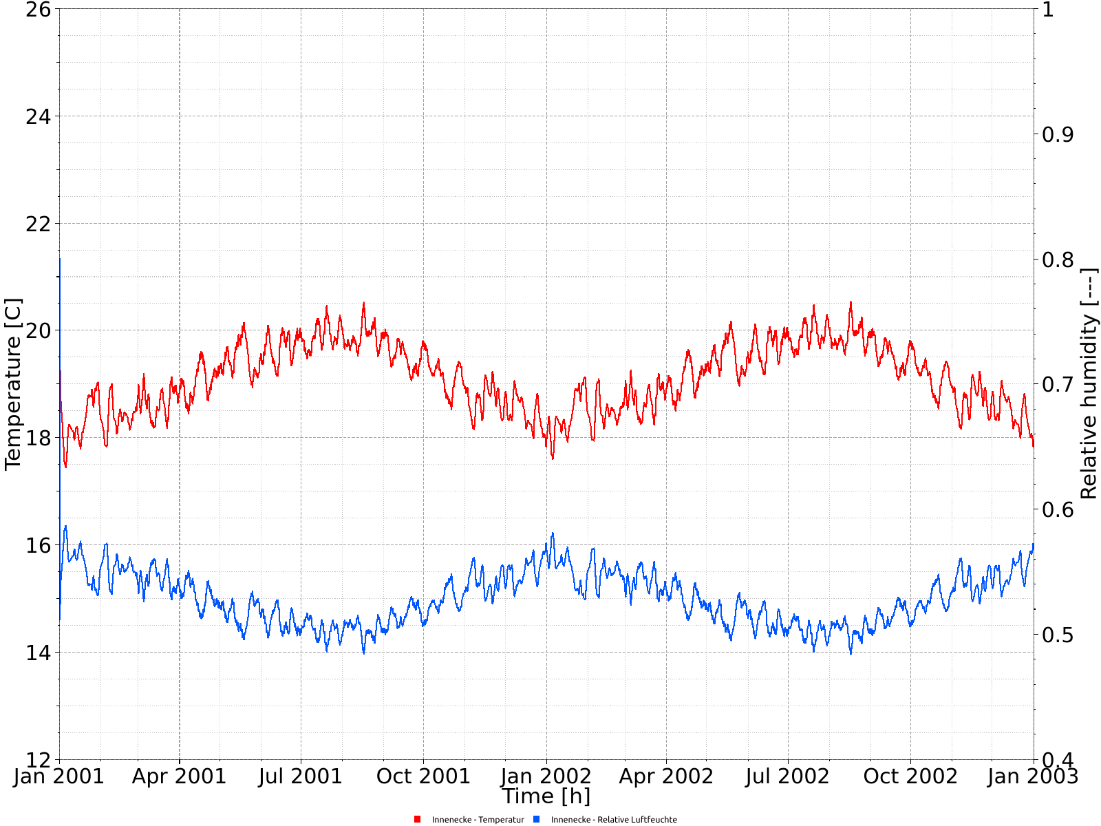
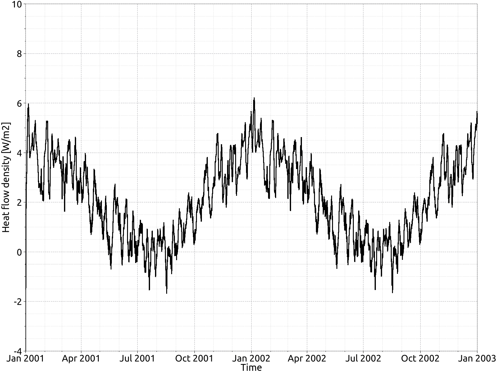
Since no critical values (approx. > 75% r.l.) are reached in this construction, it is not necessary to use a mould prognosis model. The diagram below shows the heat flow over the interior surfaces.
7. Summary
This tutorial demonstrated the steps how to create and calculate 2D constructions in DELPHIN. In the same way it is possible to generate much more complex geometries with more physical effects (air flows, moisture sources, etc.).
8. Possible further tasks
-
Modelling the construction without considering the symmetry and comparing the results.
-
Refinement of the discretisation and comparison of the results .
-
Adding an internal insulation!
-
End of the 2nd tutorial …
-